
The one perfect sorting algorithm (posted 2020-11-22)
A while ago, we discovered that there is no one perfect programming language. But is there one perfect sorting algorithm? I started thinking about that after seeing this Youtube video: The Sorting Algorithm Olympics - Who is the Fastest of them All. You may want to watch it first before continuing to read this post, as I'm going to give away the winner below.
To conveniently kill two birds with one stone, I implemented a few sorting algorithms in Python. (The second bird being learning some Python.) But as higher level languages such as Python do way too much stuff below the surface, it's pretty much impossible to see which algorithm really is faster. So I switched to C.
Before we delve into the different algorithms, first the quick takeaways:
- Sorting more stuff takes longer
- Using a newer/faster computer is faster than an older/slower one
But despite those truisms, choosing the right sorting algorithm makes a very big difference. For 10,000 items, my newest computer (2018/2020 Mac Mini) running slowest algorithm was actually a hair slower than my oldest computer (1990 Amiga 3000) running the fastest algorithm. The Mac Mini is a little over 1000 times as fast as the Amiga, but the sort takes a little under 1000 times as long. However, when sorting only 10 items, the "slow" algorithm is actually about 10 times aster than the "fast" algorithm (on the same computer). So let's have a look at the contenders.
Insertion sort
Insertion sort is like sorting a book shelf. Take one book at a time, and insert it at the correct place between the other books already on the shelf, moving those over as needed. This is extremely simple and works very well for small numbers of items, but things quickly start slowing down as the number of items to be sorted increases.
For n unsorted items, insertion sort takes about n² / 2 operations. That makes insertion sort an O(n²) algorithm in big O notation.
Quicksort
Quicksort works by selecting a "pivot" value, and then moves all items larger than the pivot to the right and all items smaller than the pivot to the left. The clever part is that this happens by swapping items, so there's no need to move large numbers of elements to make space. So Quicksort starts looking at items from the left to the right and also from the right to the left. If an item is already on the right side, it looks at the next one. As soon as it's found an item on the left that needs to go to the right and one on the right that needs to go to the left, it swaps those. When all items have been examined, we're at the point that the ones to the left are lower than the pivot and the ones to the right higher than the pivot. (Not going to worry about equal to the pivot here.) Then sort the lower-than-pivot and higher-than-pivot items separately. How? Simple, with quicksort! That's what we call recursion in the computer science business.
The performance of quicksort critically depends on the choice of the pivot. In my test program, I choose the middle value from the first, the last and the middle items to be sorted. Performance seems to be around n * log(n) with base 1.4 for the logarithm in my testing. So O(n log n) in big O notation.
Merge sort
Merge sort works by first sorting both halves of the items to be sorted (by recursively calling merge sort itself) and then merging those two sorted halves into a sorted whole. This merging works by looking at the first items of both halves, and taking the lower one. Keep selecting the lowest value from the remaining parts of each half until all items have been moved over to the place where the sorted items are kept.
A big difference between merge sort on the one hand and insertion sort and quicksort on the other hand is that the latter two work in-place, while merge sort needs extra (temporary) space to store its result. In my testing, merge sort was a hair faster than quicksort, so about the same n * log(n) = O(n log n).
Heap sort
Heap sort works by first putting the items to be sorted into a heap data structure. Conceptually, a heap is a tree, where one item sits at the top and then has zero, one or two children. The children may have one or two children of their own. Even though heaps are trees, they can be efficiently implemented as arrays. What makes a heap a heap is that a parent is always larger than its children.
We can use the special heap property to sort a bunch of items by taking that largest item from the "top" or root of the tree and putting it at the end of the data, working our way down until the heap is gone and everything is now sorted. As we do this, the heap shrinks as items take their sorted place in the array.
As we take the top item from the heap, the largest child must move up to take its place. And the largest grand child of the largest child and so on. Heap sort is also n * log(n) so O(n log n), but with a base of 1.2 rather than 1.4, so it performs significantly slower than quicksort or merge sort. But unlike quicksort it doesn't have any unusual worst cases and unlike merge sort it's in-place. Also, it's not recursive, so it doesn't take any additional system resources.
Radix sort
Radix sort is very different from the other ones, as it doesn't actually compare items with each other. Radix sort is best explained with a punch card example, as, not coincidentally, sorting punch cards was the first application of radix sort almost a century ago. A punch card sorting machine has one big "in" bin and ten "out" bins: one for each digit 0 - 9. The machine spits the cards into the different bins based on the last digit of the card's number. Then, an operator stacks up the cards again, and we repeat the whole process for the second-to-last number. Repeat with the remaining digits, and now the stack is sorted.
Radix sort is the holy grail of sorting algorithms because it takes linear time. I.e., it's O(n). So sorting ten times as many items takes ten times as long. However, it does take a lot of additional storage space for the ten bins, and life gets a lot more complex if you want to sort on text strings rather than numbers. Also, the O(n) goodness only holds as long as the key size (the length of the number or text string we're sorting on) is constant. Obviously, with many items the key size needs to increase if we want to give each item its own name or number. But for really large data sets, O(n) is king, and radix sort beats everything else.
This is how radix sort on an Amiga 3000 can beat insertion sort on a Mac Mini, for 10,000 items at least. For 10 items, insertion sort uses way fewer operations than radix sort. However, both take less than a millisecond even on the 30-year-old computer so it's hard to say which one actually runs faster in practice.
Best and worst cases
So far, we've only looked at performance for unsorted data. I used an algorithm that creates non-sequential seven-digit numbers for this. It's certainly not perfectly random, but it's random enough to resemble real-world unsorted data. But what if the data is already sorted? Or if it's reverse sorted? Or are there any other worst cases?
Insertion sort and my merge sort implementation (see below for some simple optimizations that I used) are done with sorted data after a single pass, so they are super fast in that case: O(n). Quick sort still goes through all the motions comparing items, but doesn't swap any, so it's a good deal faster than on unsorted data. Heap sort and radix sort don't run any different on sorted data.
Reverse sorted data is the worst case for insertion sort, making it twice as slow as on unsorted data because now on every one of the n passes all (average) n / 2 already sorted items need to be moved. For heap and radix sort, reverse sorted is about the same as unsorted and for merge sort, it's only a little faster than unsorted. However, quicksort has an advantage here, as on the first pass it swaps everything, so on the subsequent passes, everything is already sorted. So for quicksort, reverse sorted is almost as good as sorted.
As mentioned before, for quicksort, a lot depends on picking the right pivot. Early quicksort implementations used the last item as the pivot. That's fine on unsorted items, but a disaster for sorting already sorted data, with each pass resulting in two parts that are sizes n - 1 and 1, making the total number of passes equal to n, so now quicksort runs at O(n²). But remember, each pass is done recursively, so for non-trivial data sets, you can easily run out of stack space. Attackers can even craft malicious data sets to be sorted by a known quicksort implementation and thus crash the application doing the sorting.
Test program
This is my test program. You'll have to compile it yourself, as I don't want to be in the business of distributing executables. Do that with:
cc -o sortest sorttest.c -O3
(Or gcc instead of cc.) Note that on the Mac, if you run cc in the terminal, you'll be prompted to download the compiler and other tools, no need to waste untold gigabytes of SSD space to install Xcode. Then run the program as follows:
Usage: ./sorttest <sort> <n> [argument]
Supported sorts:
- insertion: insertion sort
- heap: heap sort
- quick: quicksort (uses median of first/middle/last items as pivot)
- quickmid: quicksort that uses middle item as the pivot
- quickins: quicksort switches to insertion sort at n <= [argument]
- merge: merge sort
- mergeins: merge sort switches to insertion sort at n <= [argument]
- radix: radix sort
n < 50 prints the items after sorting.
The merge sort merges the two sorted halves into an extra buffer and then copies that buffer back to the location of the original data. That's certainly not the most efficient way to do merge sort, so a better optimized version could run faster. However, I do check whether the last item in the first half is smaller than the first item in the second half. If so, there's no need to merge. This makes performance on already sorted data so fast. Also, under some circumstances a memory copy operation is used rather than copying each item individually, this speeds up sorting reverse sorted items.
Results
So far, I've mentioned a few results. But you may want to see some more details. (This is a Numbers spreadsheet with my results.)
My test machines, in order of performance:
- Amiga 1200 with 14 MHz 68EC020 and very slow memory (1992)
- Amiga 3000 with 25 MHz 68030 (1990)
- Amiga 1200 with 50 MHz 68060 (1995)
- MacBook Pro with 2.2 GHz Core 2 Duo running at reduced speed without a battery installed
- (2007)
- MacBook Pro with 2.4 GHz Core i5 (2013)
- MacBook Pro with 2.6 GHz Core i6 (2016)
- Mac Mini with 3.6 GHz Core i3 (2018)
I did compile the program for both 32 and 64 bit, but apart from a slight difference with insertion sort, those versions performed pretty much identically. Here's a graph of the quicksort performance on each machine:
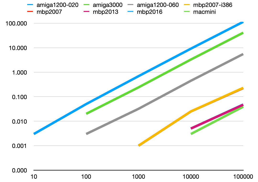
This looks pretty boring, with almost a straight (logarithmic) line as the number of items to be sorted increases. So there is no obvious point where things slow down because they no longer fit in the cache.
In order to highlight the differences between the sorting algorithms rather than the hardware differences, I decided to look at the number of compare and write operations each algorithm uses for a particular number of items to be sorted. For instance, with 8 items to be sorted, insertion sort needs 13 compares and 9 writes. For quicksort this is 34 and 8. So at 22 vs 42 operations, insertion sort is clearly faster. But at 1000 items, it's 252900 + 252900 = more than half a million operations for insertion sort and 15600 + 4800 = 20400 operations for quicksort. To more easily compare these numbers, I divide the number of operations by the number of items, so the graphs below show the number of operations per item each sorting algorithm uses for a certain number of items to be sorted. First unsorted data:
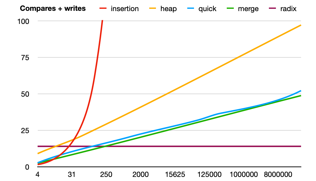
(Click on the image to cycle between compares/writes/both.) This is with data that's already sorted:
 And finally, data that's reverse sorted:
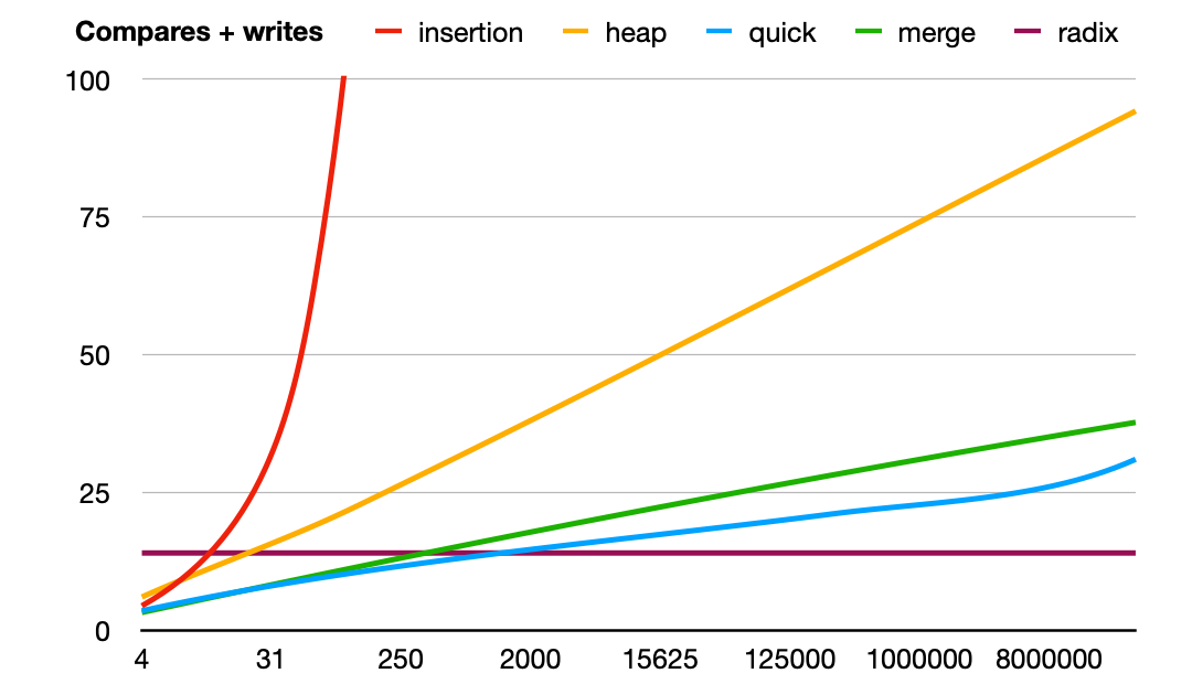
When we compare the numbers of operations with the performance in seconds, it looks like merge sort performs a bit better than the other algorithms. This could have something to do with the fact that merge sort goes through the data in order, while quicksort and heap sort jump around more.
Conclusions
In the data above it's clear that insertion sort is the fastest algorithm for very small numbers of items. It's also very easy to implement, works in-place and doesn't require recursion. Overall, radix sort is the fastest because of its O(n) property, but that advantage quickly goes away as the sort key gets longer and it requires a large amount of extra storage. So in practice, radix sort is not typically the best choice.
Quicksort and merge sort perform fairly similarly in general, but they have different strengths and weaknesses. Quicksort has the issue of choosing a pivot, but it has the big advantage that it doesn't need any extra memory. Merge sort is the faster of the two, and there are some additional optimizations possible. Merge sort can also work on data that doesn't fit in memory—in the past it was used to sort data on tape, merging the contents of two tapes to a third. Merge sort uses about the same number of compares and writes, but quicksort uses many more compares but fewer writes. A final difference is that merge sort is extremely fast on already sorted data, while for quicksort this only helps a little. But quicksort performs a bit better on reverse sorted data, while this doesn't help merge sort.
Heap sort is notably slower than quicksort and merge sort, but still more or less in the same class. The advantage of heap sort is that its performance doesn't really depend on to what degree the items are already sorted, and it's in-place and doesn't use recursion.
So to answer the question: is there one perfect sorting algorithm? No, there isn't.